Get Started

Why ggtypst?

ℹ️ One sentence summary: ggtypst is for the moments when plain plot text is not expressive enough, but a full external LaTeX workflow would be too heavy.

---

Consider these scenarios: you have a scientific plot, and now you want to:

• show your title with multiple styles, for example, the first word is red and the rest is blue
• add some special characters like Greek letters in your axis titles
• add high-quality complex math expressions as annotations in the plot
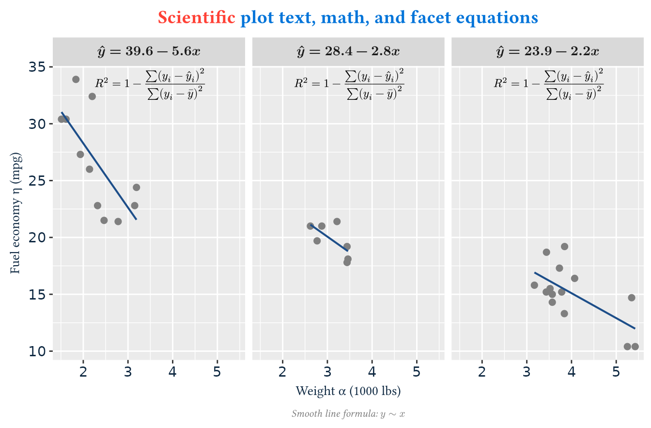
• use the corresponding regression equation as the title of each facet

How would you achieve this?

• Base ggplot2 text helpers are great for ordinary labels, but scientific and technical plots often need more than plain strings.
• You can use expression() in base R to add math. But its syntax is not natural and its functionality is limited.
• The package latex2exp helps you convert LaTeX math expressions to R expressions. But its functionality is also limited by expression().
• The package ggtext allows you to use Markdown and HTML tags to style your text. But it doesn’t support complex styles and math.
• tikzDevice/ggtikz allows you to use LaTeX. But it is too complex to use and must rely on external TeX toolchains, which are very heavy.
• …

So is there a simple, lightweight, easy-to-use solution? Yes, that’s why ggtypst is here!

---

Typst is a modern markup language and typesetting engine written in Rust. You can write source text such as *bold*, _italic_, #linebreak(), or $ sum_(i=1)^n x_i $, and Typst turns it into polished rendered output. It is fast, simple but powerful, solving these pain points perfectly and elegantly.

ggtypst uses Typst’s Rust engine as the rendering backend and offers a series of functions to fit ggplot2 workflow. With ggtypst, you don’t need to leave your ggplot2 workflow, don’t need to rely on external LaTeX or Typst, and can easily solve all the above use cases.

Click to see the code

eq_labels <- by(mtcars, mtcars$cyl, function(df) {
  fit <- lm(mpg ~ wt, data = df)
  coef <- unname(coef(fit))

  sprintf(
    "hat(y) = %.1f %s %.1f x",
    coef[1],
    if (coef[2] < 0) "-" else "+",
    abs(coef[2])
  )
})

ggplot(mtcars, aes(wt, mpg)) +
  geom_point(color = "grey50", size = 2) +
  geom_smooth(method = "lm", formula = y ~ x, se = FALSE, linewidth = 0.7, color = "#1D4E89") +
  facet_wrap(vars(cyl), nrow = 1, labeller = as_labeller(eq_labels)) +
  annotate_math_typst(
    r"(R^2 = 1 - sum(y_i - hat(y)_i)^2 / sum(y_i - macron(y))^2)",
    x = 3.5,
    y = 33.5,
    size = 10
  ) +
  labs(
    title = r"(#text(fill: red)[Scientific] #text(fill: blue)[plot text, math, and facet equations])",
    x = "Weight α (1000 lbs)",
    y = "Fuel economy η (mpg)",
    caption = "Smooth line formula: $y ~ x$"
  ) +
  theme(
    plot.title = element_typst(size = 16, face = "bold"),
    axis.title.x = element_typst(size = 12, colour = "#102A43"),
    axis.title.y = element_typst(size = 12, colour = "#102A43"),
    axis.text = element_typst(size = 11, colour = "#102A43"),
    strip.text = element_math_typst(size = 12, face = "bold"),
    plot.caption = element_typst(size = 9, color = "grey50", face = "italic")
  )

Installation

Install ggtypst from R-universe first so you can use the prebuilt package and avoid compiling Rust locally:

install.packages("ggtypst", repos = "https://yousa-mirage.r-universe.dev")

If you need the latest development version from GitHub, you can install it from source:

install.packages("remotes")
remotes::install_github("Yousa-Mirage/ggtypst")

Because the GitHub installation builds the Typst backend in Rust, you need rustc and cargo on your system to compile it. Particularly on Windows, you must use the x86_64-pc-windows-gnu toolchain. Regardless of how you install ggtypst, you don’t need a separate local Typst or LaTeX installation to use it.

First plot

A quick example is like this:

ggplot(mtcars, aes(wt, mpg)) +
  geom_point(color = "grey50") +
  annotate_typst(
    typst_code = "*Hello from Typst!* #linebreak() $sum_(i=1)^n x_i$",
    x = 4.8,
    y = 32,
    size = 14,
    color = "#1D4E89"
  ) +
  labs(
    title = "A first ggtypst plot",
    x = "Weight (1000 lbs)",
    y = "integral_0^1 x^2 dif x = 1/3"
  ) +
  theme_minimal(base_size = 12) +
  theme(
    plot.title = element_typst(size = 16, face = "bold.italic", colour = "#102A43"),
    axis.title.y = element_math_typst(size = 14, colour = "#1D4E89")
  )

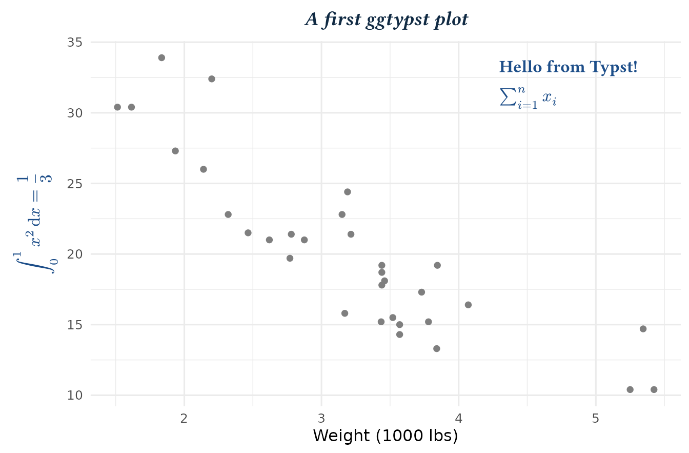
This shows the core usage of the package:

1. First, we use annotate_typst() to add a Typst label containing text and inline math.
   • * ... * marks bold text.
   • #linebreak() inserts a line break.
   • $...$ marks inline math.
   • We specified the plot location, text size and color by other arguments.
2. Then, we want to render the title and axis titles with Typst.
   • We write a common title, and then render it with Typst through element_typst().
   • We want to use a math expression as the y-axis title, so we write the Typst math source code in labs() and then use element_math_typst() to render it.

When to use annotate, geom, and element

Use the three function families according to where the rendered content comes from.

Function family	Best for	Typical use
annotate_*()	one manually placed label	a callout, note, or equation
geom_*()	one label per row of data	point labels, grouped labels, math annotations
element_*()	theme text	titles, subtitles, axis text, strips, legends

R raw strings

Typst and LaTeX source strings may contain lots of " and \. In ordinary R strings, these characters need to be escaped like "\\frac{a}{b}". Introduced in R 4.0.0, R raw strings let you write these special characters directly without escaping.

ℹ️ You should ALWAYS use the raw string r"( ... )" in your Typst and LaTeX source:

r"(*bold text*)"
r"($"a text in math" sum_(i=1)^n x_i$)"
r"(\frac{a}{b})"

Text, Typst math, and MiTeX math

ggtypst supports three related but different kinds of content.

Typst markup content

Typst is a language for typesetting documents. It has two modes: the markup mode and the function mode. In markup mode, you write plain text with Typst markup syntax, similar to writing Markdown. For more details, please see the Typst documentation. It’s very easy to learn and use.

Use annotate_typst(), geom_typst(), or element_typst() when the label is mostly text. For example:

annotate_typst(
  typst_code = r"(*bold text*)",  # `*...*` means bold text
  x = 1,
  y = 1
) +
annotate_typst(
  typst_code = r"($a^2 + b^2 = c^2$)",  # `$...$` means inline math
  x = 2,
  y = 2
) +
annotate_typst(
  # In the line below, "Red text" is styled with `fill: red`, "default text" is styled with italic, and `+` is with default style.
  typst_code = r"(#text(fill: "red")[Red text] + _default text_)",
  x = 3,
  y = 3
)

Yeah, actually you can write any legal Typst content in typst_code, including math, styled text, layouts, and functions. You can even write a full Typst document in typst_code, as long as the source string is legal Typst content. They will be directly rendered by Typst.

Native Typst math

You can use *_math_typst() when you want to write math directly. They are wrappers around *_typst() that use the typst_math_code argument instead of typst_code.

annotate_math_typst(
  typst_math_code = r"(sum_(i=1)^n x_i)",
  x = 1,
  y = 1
)

$ ... $ or $...$ will be automatically added around your math code to make sure it is rendered as a math expression. The difference is, $ ... $, which is default, means display math, while $...$ means inline math. You can use the inline argument to control which to use.

Of course, you can also use annotate_typst() and write your math code in $ ... $ or $...$. *_math_typst() are just more convenient wrappers.

One more important benefit of Typst is that you don’t need to have a math font installed on your system to render math expressions. Typst has embedded the New Computer Modern Math font in binary, so you can render math anywhere and anytime.

MiTeX-backed LaTeX math

You can use annotate_math_mitex(), geom_math_mitex(), or element_math_mitex() if you are more familiar with LaTeX math syntax or when your input is already in LaTeX. ggtypst converts LaTeX math into Typst math by MiTeX in the Rust backend. According to their documentation, this conversion is stable and supports a wide range of LaTeX math syntax.

annotate_math_mitex(
  latex_math_code = r"(\frac{1}{2} + \sqrt{3})",
  x = 1,
  y = 1
)

annotate_*(): one-off plot annotations

annotate_*() is the easiest place to start because it behaves like a normal manual annotation layer. Use this function family when you just want to add one rich text note or math equation at a specific position.

ggplot(mtcars, aes(wt, mpg)) +
  geom_point(color = "grey65") +
  annotate_typst(
    typst_code = r"(Some plain text)",
    x = 2,  # You must specify the x and y position manually
    y = 15
  ) +
  annotate_typst(
    typst_code = paste(
      r"(*Fuel economy* #linebreak())",  # text with bold markup and line break function
      r"(#text(fill: rgb("#1D4E89"))[Typst text] +)",  # text with fill color
      r"($integral_0^1 x^2 dif x = 1 / 3$)"  # inline math
    ),
    x = 4,
    y = 33,
    size = 12,
    color = "#102A43"
  ) +
  annotate_math_mitex(
    latex_math_code = r"(\eta = \frac{mpg}{wt})",  # LaTeX math code
    x = 5,
    y = 25,
    size = 14,
    color = "green",
    face = "bold"
  ) +
  theme_minimal(base_size = 12)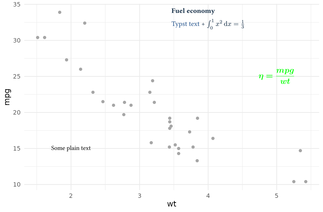

geom_*(): data-driven labels

geom_*() turns Typst source strings into a true data layer. Each row gets its own rendered label and can map aesthetics like colour, angle, and face. Use this family when:

• you have many labels to render
• labels come from rows in a data frame
• each label may have different styling
• you want Typst output to behave like other ggplot2 geoms

labels <- data.frame(
  wt = c(2, 3, 5),
  mpg = c(33, 25, 15),
  label = c(
    r"(*Toyota Corolla* #linebreak() 33.9 mpg)",
    r"(*Fiat 128* #linebreak() nimble + efficient)",
    r"(*Maserati Bora* #linebreak() $v_8$ flagship)"
  ),
  colour = c("yellow", "#3A86A8", "#7A1E48"),
  face = c("italic", "bold.italic", "bold")
)

ggplot(mtcars, aes(wt, mpg)) +
  geom_point(color = "grey80", size = 2) +
  geom_typst(
    data = labels,
    aes(wt, mpg, label = label, colour = colour, face = face),
    size = 12,
    show.legend = FALSE
  ) +
  scale_colour_identity() +  # this is needed for colour mapping
  theme_minimal(base_size = 12)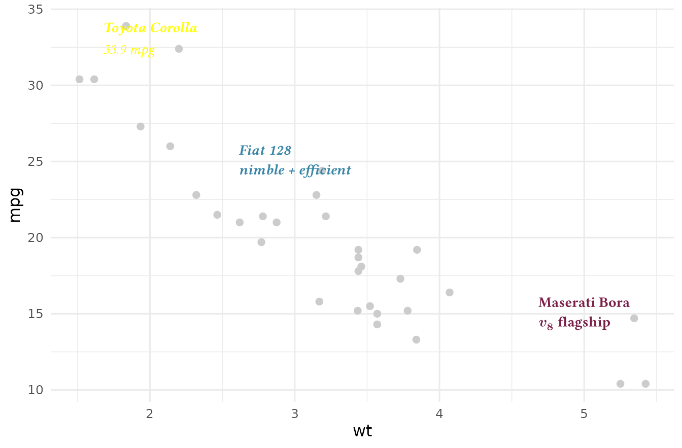

However, be careful not to use geom_typst() to render more than 50 label rows, as it will not only slow down rendering but also make your plot hard to read. For more details on performance, see the benchmark result.

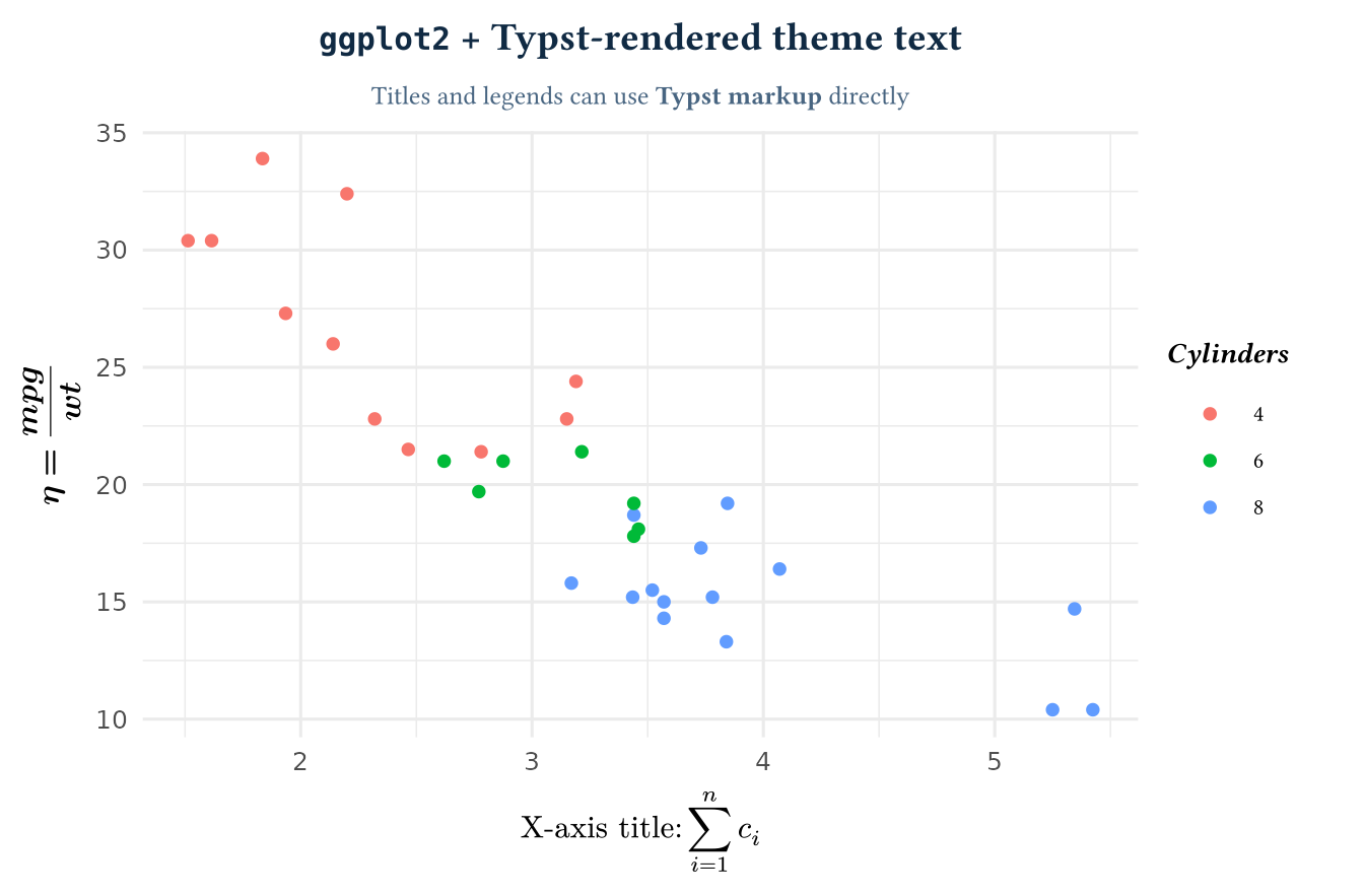
element_*(): Typst in theme elements

element_*() is used to render the text of theme elements with Typst. By element_*(), you can place rich text, special characters, and math equations in your plot titles, subtitles, axis titles, legend text, and facet strips.

Imagine that your ggplot2 title is a math matrix, while each facet label is the special regression equation!

ggplot(mtcars, aes(wt, mpg, colour = factor(cyl))) +
  geom_point() +
  labs(
    title = r"(`ggplot2` + Typst-rendered theme text)",
    subtitle = r"(Titles and legends can use *Typst markup* directly)",
    x = r"($"X-axis title:" sum_(i=1)^n c_i$)",
    y = r"(\eta = \frac{mpg}{wt})",  # LaTeX math is OK
    colour = r"(_*Cylinders*_)"
  ) +
  theme_minimal(base_size = 12) +
  theme(
    plot.title = element_typst(size = 16, face = "bold", colour = "#102A43"),
    plot.subtitle = element_typst(size = 11, colour = "#486581"),
    axis.title.x = element_math_typst(size = 13),
    axis.title.y = element_math_mitex(size = 13, face = "bold"),
    legend.title = element_typst(size = 12),
    legend.text = element_typst(size = 10)  # render legend labels with Typst
  )

Next steps

From here, you can explore:

• the function reference for annotate_*(), geom_*(), and element_*()
• the contributing guide if you want to understand the R/Rust architecture
• and practice ggtypst in your RStudio/Positron/VS Code